Intro

On this page, a few tools and methods gathered over the past years of practice as a pythonist (it would have been useful to know this from start…). This page might prove to be worth reading for people dealing with measured data, equations, modelling or teaching. The theory behind the scenes is not tackled: only the practical aspects are shown with minimal working examples.

On the agenda:

• data interpolation
• data resampling
• function integration
• integration of interpolated data (yes.)
• equation solving
• sensivity analysis
• metamodeling
• parallelisation

Data interpolation

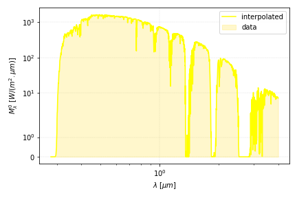
In this section, we will use the ground level solar spectrum radiation data provided by the NREL (ASTM AM 1.5). It includes the absorption of radiation by gases in the atmosphere.

The aim is to create an interpolation function in order to obtain the values at different abscissa using scipy.interpolate. The main features of the code are presented below and should roll gently with the comments:

import pandas as pd # pandas will help reading the xls file containing the data
import scipy.interpolate # interpolation package 

# let us read the radiation data 
df = pd.read_excel('ASTMed.xls')
df['lambda']=df['lambda']/1000 # convert to micrometers
df['global']=df['global']*1000 # convert to W/m2/micrometer

# measured data
x = df['lambda'].values
y = df['global'].values
# create the interpolation function
fc_interp = scipy.interpolate.interp1d(x, y)
# compute the interpolated values (in this cas the exact ones)
interpolations= fc_interp(df['lambda'].values)

print("Radiation at 0.55 micrometers", fc_interp(0.55), 'W/m²/um')

That’s about it, the rest is plotting! You can get the data in .xls file format and the code here

Resampling data

In many fields, being able to resample data is of practical use. For instance if you have measured data at 1 hour interval and require values every 10 minutes. No need to worry about creating your own interpolation routine: Using exactly the same procedure described above, you can proceed as follows.

import numpy as np # numpy import for convenience

# measured data
x, y = df['lambda'].values, df['global'].values
# create the interpolation function
fc_interp = scipy.interpolate.interp1d(x, y)

#let us define a new interval every 0.5 micrometer between the bounds
wavelengths=np.arange(min(x),max(x), 0.5)
# get the resampled radiation data
resampled_radiation = fc_interp(wavelengths)

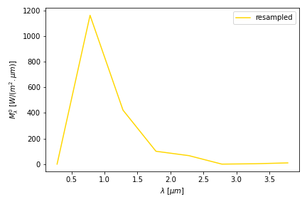
(looks weird, indeed… usually you resample the other way around: with more data!)

Numerical integration

Life is beautiful since the invention of numerical integration. It is even more so since it was made possible with less than 10 lines of code. Using the same physical problem as the previous example, let us now compute the black body radiation emitted by the sun over its spectrum.

We will therefore use Planck’s law for the black body emission, which forms more than half the code required, as you can see for yourself below.

import scipy.integrate as integrate # import the integration method

# Planck's emission law depending on wavelength x [micrometers] and temperature T [K]
# scaled for the flux intensity reaching the earth
def sun_radiation(x,T):
    #a few constants
    h=6.62*1e-34 # Planck's constant
    k=1.3805*1e-23 # Boltzmann's constant
    c=3*1e8 # light velocity
    C1=2*np.pi*h*c**2*1e24 # 1e24 = conversion m^4->µm^4
    C2=h*c/k*1e6 # 1e6 = conversion m->µm
    S_sun=4*np.pi*(6.957*1e8)**2 # surface of sun
    S_sunEarth=4*np.pi*(149.598*1e9)**2 # surface of the sphere with radius sun->earth
    return C1*x**(-5)/(np.exp(C2/(x*T))-1)*S_sun/S_sunEarth

k = np.arange(0.05, 50, 0.001) # wavelength range in micrometers
Tsun=5800 # K
#now  a little trick using Wien's law: 
lambda_m=2898/Tsun 
# ... indeed most of the energy of the black-body spectrum is comprised 
# between 0.5 and 5 lambda_max, hence no need for a larger integration range
E_sun= integrate.quad(lambda x: black_body_radiation(x,Tsun), 0.5*lambda_m, 5*lambda_m)[0]
print("radiation of the black body", E_sun, " [W]")

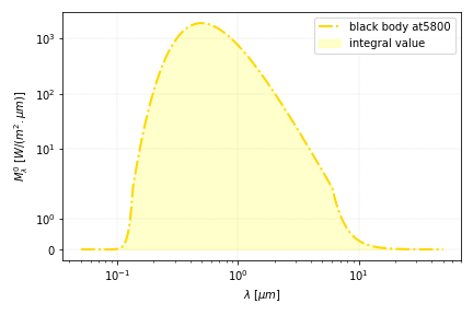
(finding a value above 1000 W is ok since we consider here the extraterrestrial sun radiation - don’t complain to Max Planck)

Combine: Integrate your measured data

It is sometimes handy to integrate measured data (e.g. power over time → energy).

Imagine that for some reason, you want to compute the energy comprised in the ASTM solar data of the first example. You can either do it directly in the .xls file provided, using the rectangle integration method, or follow the tutorial presented here.

You may have noticed that numerical integration requires a function to be integrated (that is: black_body_radiation() in the script above). Very handily, the interpolation function proposed in the previous section provides fc_interp() which allows for the determination of the value of the function at any abscissa (within the data, no extrapolation).

import scipy.integrate as integrate #
E_sun= integrate.quad(lambda x: fc_interp(x), min(x), max(x))[0]
print("and the solar energy spectrum contains...", E_sun, " Watts!")

(if you find a value above 1000 W, call the NREL and complain)

Nota bene: Saw-toothed data samples may lead to the display of some warning-verbose. You may want to double-check the order of magnitude of the value obtained with a good old rectangle method of integration like integral=np.sum(f(x))*dx.

Solving equations

Equations are suddenly much simpler when computers solve them for us. You will find two examples below to kick-start your code.

Computing the wet bulb temperature (one unknown)

The wet-bulb temperature is defined in the equation below as a function of itself:

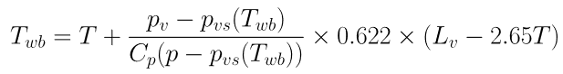
A simple way to solve this (complicated) equation it is to create a function of Twb that return Twb-f(Twb)=0 and to ask the specialised procedure fsolve to do it for us:

import numpy as np # for generic math/array operations
from scipy.optimize import fsolve # queen of solving procedures

# a function for the vapour pressure at saturation pvs(T)
def pvs(T):
    a,b=0.07252,0.0002881
    c,d=0.00000079,611
    return d * np.exp(a*T -b*np.power(T,2) + c*np.power(T,3))

# the function that will allow finding Twb depending on temperature T and vapour pressure pv
def fc_Twb(Twb, T, pv):
    Cp, p, Lv = 1.006, 101325, 2400
    return - Twb +T+ (pv-pvs(Twb))/(Cp*(p-pvs(Twb)))*0.622*(Lv-2.65*T)

# let's define the temperature and vapour pressure conditions
Ta = 40 # air dry bulb temperature
pv=0.3*pvs(Ta) # let us go for 30% relative humidity

# initial guess for the solution
Twb_guess = Ta-10 # usually Twet-bulb is on the left of Tdry

# solving with fsolve (note the first argument is the unknown and the others are given separately)
# compute the wet-bulb temperature:
Twb = fsolve(fc_Twb, Twb_guess, args=(Ta, pv))
print("wet bulb temperature", Twb)

You can now replace the function fc_Twb by the one of your choice and ask scipy to fsolve it for you!

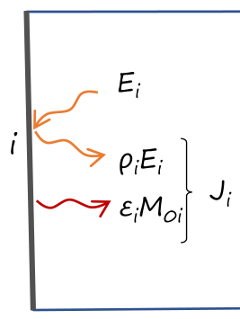
n unknowns: The radiosity method

Suppose we want to compute the total fluxes between the internal faces of a cube. We will use the radiosity method, that consists in computing the net radiative flux between surfaces.

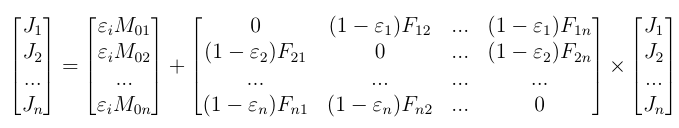
The radiosity J is the total radiative flux emitted and reflected by a face:

The system to be solved depending on the temperatures, emissivities and view factors between faces writes as:

Let us imagine that the cube faces are at 10°C, while the bottow is maintained at a cool -10°C. Faces are numbered as per the sketch below.

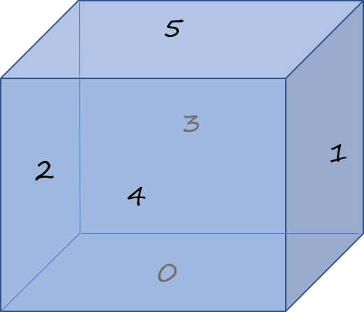
The code writes as follows. The major part of it is dedicated to the (dirty) filling of the view factor matrix.

import numpy as np
from scipy.optimize import fsolve

# view factors for opposite and adjacent faces in a cube
Fadj, Fopp=0.200044, 0.199824
# view factors matrix
Fij=np.zeros((6,6))
# fill the matrix
for i in range(6):
    for j in range(6):
        # adjacent faces
        if not i==j:
            Fij[i,j]=Fadj
        # opposed faces 0-5 / 1-2 / 3-4
        for z in [(0,5), (1,2), (3,4)]:
            a,b=z
            if (i==a and j==b) or (i==b) and (j==a):
                Fij[i,j]=Fopp

def fc_radiosity(J, T, Fij):
    sigma,epsilon = 5.67*1e-8, 0.9
    return -J + sigma*epsilon*T**4 + (1-epsilon)*np.dot(Fij,J)

# the faces are at +10C...
T=np.ones(6)*(10)
# ... the bottow at -10C
T[0]=-10
# convert the array to Kelvin
T=T+273.15

# initial values for Ji
J_init=np.ones(6)*100
# solve for Ji
J=fsolve(fc_radiosity, J_init, args=(T, Fij))
print("Radiosities [W/m2]", J)

#total incident radiation per face
E=np.dot(Fij,J)
print("Total radiation [W/m2] ", E)

The snippet above can be adapted to other configurations, provided that the view factors are known (code file).

Sensitivity Analysis

Some models are complex and require an important number of parameters. It is often useful to know which of the parameters are the most influential on the observed output of the model (e.g. for building simulation: is it the wall insulation level or the properties of windows that affect most the energy consumption?). In the case of optimisation, knowing the influential parameters allows for instance to concentrate the computational effort on the meaningful inputs with regard to the considered output.

Dedicated mathematical methods establishing the ranking of parameters do exist (phew!). Most of them are based on the observation of the output of a limited number of well-chosen simulations of the model. We will use the SAlib sensitivity analysis package and especially Morris’ method, which is easy to understand (the average effect of each parameter variation and the standard deviation between two simulations are observed).

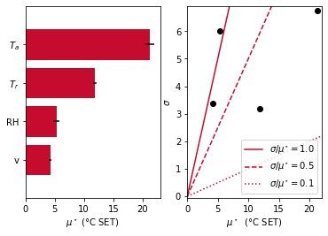
The package pythermalcomfort will serve as an example here: we will use it in order to determine which ambient parameters (air velocity, radiant temperature, air temperature, relative humidity) are the most influential on the Standard Effective Temperature (SET) comfort index.

import numpy as np
from pythermalcomfort.models import set_tmp
from SALib.plotting.morris import horizontal_bar_plot, covariance_plot
from SALib.analyze import morris
from SALib.sample.morris import sample

# Define the model inputs
problem = {
    'num_vars': 4, # nb variables
    'names': [r'$T_a$', r'$T_r$', 'v', 'RH'], # variable names
    'bounds': [[10,40], # lmin/max for each variable
               [10,40], # radiant temperature
               [0.1,1], # air velocity
               [10,90]] # relative humidity
}
# generate samples
N_repetitions=50
num_vars=problem['num_vars']
# number of function evaluations we are  going to perform:
print("Evaluations ", N_repetitions*(num_vars+1))
# prepare evaluations
param_values= sample(problem, N_repetitions, num_levels=4)
Nmax=max(np.shape(param_values)) # values as output

# the call looks like
# set_tmp(tdb=Tair, tr=Trad, v=v, rh=hum, met=1.2, clo=.5)
# so let's create the arrays for metabolic rate and clothing:
array_met=np.ones(len(param_values))*1.2
array_clo=np.ones(len(param_values))*0.5
# ... and stack them to the param_values matrix
param_values_with_metclo=np.hstack([param_values, array_met[:,None],array_clo[:,None]])

# prepare the output array
Y=np.empty((Nmax)) 
# do the function evaluation
for i,p in enumerate(param_values_with_metclo):
    Y[i]= set_tmp(*p)

# Perform analysis with the results in array Y[i]
Si = morris.analyze(problem, param_values, Y, conf_level=0.95,print_to_console=True, num_levels=4)

The code generates following output, showing that the air temperature is the most influential parameter within this range of evaluation. The relative humidity has a smaller effect but it lies on the first bisector, meaning its average effect is of the order of magnitude of the standard deviation: non-linearity possibly arises in the model or interactions between parameters may occur.

Metamodeling: Kriging

Some models are costly in terms of simulation time. When numerous runs of the model with differents sets of parameters are required, the creation of a metamodel is often an interesting means of reducing the computational cost.

Creating a metamodel is much like adding a polynomial fit or a trend curve on your favorite spreadsheet software, excepted that there can be numerous input parameters. It can hence be seen as an interpolation method (and actually it is renowned for its efficiency in field interpolation).

The kriging procedure of the much appreciated package SMT will be used in the sequel. Since you may already have installed/used the pythermalcomfort package with the example above, we will create a metamodel for the SET.

Imagine that for future use, we want to avoid the computation of the SET comfort index with set_temp() from pythermalcomfort (suppose it takes too long) and still be able to obtain its value depending on the air temperature and the radiant temperature. We will set up such a metamodel in the following code lines:

# boundaries of the air and radiant temperatures
Tmin,Tmax=10,40 # air temperature
Trmin,Trmax=20,40 # radiant temperature
xlimits = np.array([[Tmin, Tmax], [Trmin, Trmax]])

#metamodel set up
nb_LHS = 100 # number of evaluations
# type of sampling 
sampling = LHS(xlimits=xlimits, criterion='c')
# sample data set
xt = sampling(nb_LHS)
yt=np.empty([nb_LHS]) # prepare array for filling

# air velocity (m/s) and relative humidity (%)
vair,hum=0.15, 55
for k in range(len(xt)):
    Ta,Tr,v,hum=xt[k,0], xt[k,1], vair, hum # put it in a readable way
    yt[k]=set_tmp(tdb=Ta, tr=Tr, v=v, rh=hum, met=1.2, clo=.5) # evaluate the function

# prepare the metamodel
sm = KRG(theta0=[1e-3], corr='abs_exp')
sm.set_training_values(xt, yt)
sm.train()  # --> this is the costly part

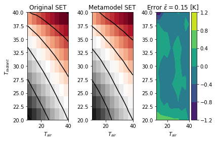
Once the metamodel is trained, it can be used for prediction with the simple instruction sm.predict_values(Tair, Tradiant). The full code allows to produce following output, with a reasonable 0.15 [K] of average error on the prediction of the SET versus the original one.

Go parallel

Parallelism has become very affordable and easy over the years. Still using the pythermalcomfort package, a minimum working example of parallelisation is provided. It can be modified and applied to any other function call (running EnergyPlus, reading files, computing averages etc.).

import numpy as np
from pythermalcomfort.models import set_tmp
from joblib import Parallel, delayed

# let's do a couple of runs
N_evaluations=100000

# prepare the arrays for the example
array_Ta=np.ones(N_evaluations)*20
array_Tr=np.ones(N_evaluations)*25
array_v=np.ones(N_evaluations)*0.1
array_RH=np.ones(N_evaluations)*50
array_met=np.ones(N_evaluations)*1.2
array_clo=np.ones(N_evaluations)*0.5
param_values=np.hstack([array_Ta[:,None],array_Tr[:,None],array_v[:,None], array_RH[:,None], array_met[:,None],array_clo[:,None]])

#the parallel execution is below this line
if __name__ == '__main__':
    num_cores = 4
    SET_array=Parallel(n_jobs=num_cores)(delayed(set_tmp)(*p) for p in param_values)

Note - If the function to be parallelised is not really computationally expensive (as is the case here), you may experience little to no speed-up or even an increase of the execution time. Parallelise wise!

An alternative using pool including a fancy progress bar is proposed hereinafter (note the usage of tqdm and the function call):

from tqdm import tqdm # package for the progress bar
from multiprocessing import Pool
if __name__ == '__main__':
    num_cores = 4
    with Pool(processes=num_cores) as p:
        SET_array=p.starmap(set_tmp, tqdm(param_values, total=len(param_values)))